Valuable Excel Functions: VLOOKUP

One of the most powerful, yet overlooked, features in Excel is the VLOOKUP function. VLOOKUP itself enables users to search for a value in one column and return a corresponding value from another column. The function reduces the need for manual scanning of data which is especially helpful in large datasheets. With VLOOKUP, you can simplify the way you organize, analyze and interpret data. For example, let’s say you have two tables and would like to cross reference certain records, or you have one large table and would like to pull out specific information for a “what if” scenario. In both of these cases, VLOOKUP proves invaluable.

The syntax of the command can be a bit of a mouthful, but it’s easy enough once you get the hang of it. Let’s break it down.

VLOOKUP(lookup_value, table_array, col_index_num,[range_lookup])

• lookup_value: The value to search for in the first column of the table.
• table_array: The range of cells containing the data you want to search.
• col_index_num: The column number in the table from which to retrieve the value. Note: the leftmost column is number one, the second leftmost is two and so on.
• range_lookup: This optional argument specifies whether you want an exact match (FALSE) or an approximate match (TRUE). The default is TRUE.

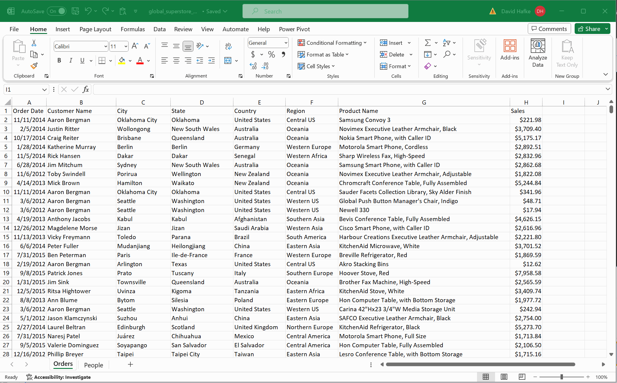
Consider the following table of order records for a global e-commerce vendor.

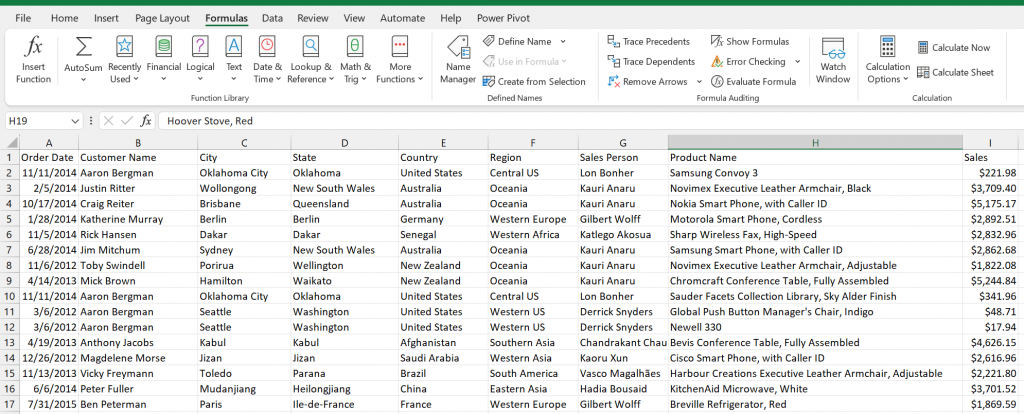
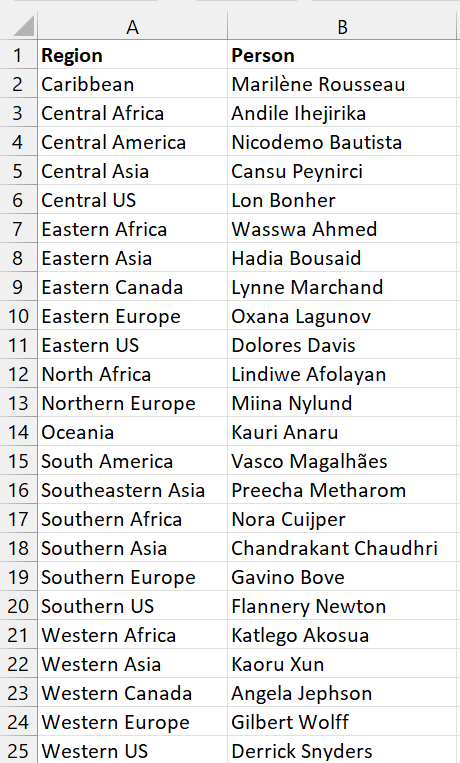
Now let’s say you wanted to add the salesperson for each region as indicated below.

With VLOOKUP, you can do this in three easy steps:

1. Simply add a new column for the salesperson.
2. Enter the VLOOKUP command in the top data cell. In this case: VLOOKUP(F2,People!$A$1:$B$25,2,FALSE). Note the use of absolute cell references ($A$1:$B$25). This is important for the next step.
3. Copy the formula to each empty cell below.

That is all there is to it!

A few final tips and tricks:

1. An alternative to using absolute references as mentioned above is to use a “Named Range,” by selecting your table and then clicking “Define Name” in the Formulas tab of the ribbon.
2. If you’re unexpectedly getting #N/A as a result, double check the data type of the cells and ensure there are no typos including superfluous spaces.
3. Consider using the IFERROR function to display a customized message rather than the ugly #N/A error if your cell doesn’t hit a match.

Mastering the VLOOKUP feature in Excel is a valuable skill for anyone working with data. Whether you are a business analyst, financial professional or simply managing personal finances, understanding how to efficiently retrieve and analyze data using VLOOKUP can significantly streamline your workflow. As you explore its capabilities and experiment with different use cases, you’ll discover the versatility and power that this function brings to your Excel toolkit.